Basic VCF Algorithm

General ideas.

This presentation assumes that each pixel has only one scalar value, such as in grayscale images. The same concepts can obvioulsy by applied to multi-channel pixels to compress color images.

The proposed algorithm's cornerstone is to uses a visually understandable degradation of image parts. The general idea is to divide the image in a number of parts, called cells in the present document, and then give the best possible representation of each in the smallest number of bits.

For that, we choose to use a blurred approximation of the cells, as because we think this is the most visually acceptable degradation for most images¹. The simplest cell approximation is a cell where all pixels have the same value, and the optimal value for that is the mean of all values of the original pixels: the cell value. This approximation will be refered to as "coarse detail level", or "top" level. This approximation (which we don't expect to be a visually acceptable degradation of the original image, BTW) represents the whole cell with only one parameter.
The next step will be to give a slightly better approximation using a few more parameters. And so on, we will have better and better representations of the cell, using more and more parameters, until we reach the so-called "fine details level", or "bottom" level, where the representation is identical to the original image.
All we have to do now is to choose what level of detail is acceptable for each cell by computing the distance² between the cell approximation and the orignal, and by doing that find the smallest number of parameters needed to describe the cell.
Simple ;-)

Trees of cells: the Crystallization.

One strong constraint of the above presentation is to reach the original image. This is often ignored by low bit-rates compression algorithm. However, this is absolutely needed for high-quality images.

The only exact representation of the original set of P pixels using the smallest number of parameters is the original image itself, using P parameters. (which is not as obvious as it sounds)

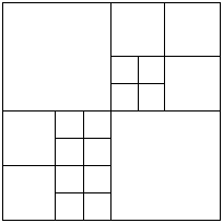
The VCF algorithm uses only square cells of N x N pixels. At each level the upper cell is divided into 4 children cells of N/2 x N/2 pixels. Hence the need of 4 parameters to describe each lower level cell.

Such a division is called "transition" in this paper. The transistions are simply coded by a bit: 1 means there is a transition, 0 means there is no transistion. This way of coding the transitions of square cells in a tree using binary digits is optimal to describe an image area of any shape.
When a transition does not occur, we paint the cell using the cell pixel value.

If we choose to read the squares top to bottom and left to right, the example in the above figure will be coded as:
1 0 10010 0101 0
This example assumes that we know which level is the last one, in order to avoid coding "0000" for each bottom-most cell. This cell in the example will be coded into 12 bits and 19 pixel values instead of 8x8=256 pixel values: a 12:1 compression rate.

The loss parameter.

Now we have to decide how much we want the approximation to be approximative. For that, we evaluate how much we loose in the image by using a N x N cell instead of 4 N/2 x N/2 cells, for each transition. This value can be calculated by substracting to the distance of the N x N cell each of the 4 distances of the N/2 x N/2 cells (this is why we don't want to use the MSE: we need actual distances, not mean values). This value is called "pertinence to the transition" in VCF terminology, and its unit is the same as the square of a pixel value.

If a transition is pertinent at a finer level, we must force the transistions at coarser levels in order to allow the finer transition to occur. That is why we want to consider for each cell the pertinence of all its children (the highest pertinence of the cell and all its children) instead of only the cell of pertinence itself. It should be noted that the pertinence can never be negative, because each transition is alway an improvement using optimal values (means).

For the test implementation, we will use the same loss for all cells of the image, and the loss will have the same unit as a pixel value. The square of this loss will be the lowest pertinence we want to keep: lower values will give better images. JPEG uses the concept of "quality" instead, where higher valuer give better images.

Implementation.

We have now a parametric lossy description of the original image using only these few informations:
- number of top level cells in the width of the image.
- number of cell levels in the image (for implicit fine level transitions).
- the transitions tree.
- the non-transitions pixel values.

The algorithm for compression and decompression has been explained in less than 1000 words, and the test implementation done in C has 500 lines for compression and 150 lines for decompression. This is a deterministic algorithm with no convergence condition. The computational power needed is close to 2 multiplication-addition per pixel for compression and 1 for decompression, which is in the order of magnitude of memory-to-memory copying. The memory usage besides the size the image itself is very low, about the size of two top level cells.

The cell approximation is not the best approximation we could have used, but this is the simplest and the easiest to implement to test the algorithm. Better cell approximations will be disscussed later in this paper. Particularly, we expect the two source of artefacts to be the discontinuity between the border of two adjascent cell, leading to sub-optimal rendering of gradients.
Still, we expect this algorithm to behave as discussed and to give some promissing information about the improvements that could be made.

¹ For special applications, it might be best to use a different approximation. Compression of fingerprints comes to mind.
² The distance between two images is calculated in this document by adding the square of the difference of each pixel in the first image and the pixel at the same position in the second image. Usual distance calculation take the square root of this sum, which is basically the same. Another distance mesure (MSE) divides this sum by the number of pixels; we will explain later why the MSE is not good for VCF.

prev toc next

last modification: March 2002
(C) Eric GAUDET, 2002